Dávid Hanák
Budapest University of Technology and Economics
Dept. of Computer Science and Information Theory
The abstract description language defined by the theory may also be interpreted by a computer program. This paper deals with the problematic issues of putting the theory into practice by implementing such a program. It introduces a concrete syntax of the language and presents three programs understanding that syntax. These case studies represent two different approaches of propagation. One of these offers exhausting pruning with poor efficiency, the other, yet unfinished attempt provides a better alternative at the cost of being a lot more complicated.
Constraint Logic Programming (CLP, also referred to as Constraint Programming, CP) [1] is a family of logic programming languages, where a problem is defined in terms of correlations between unknown values, and a solution is a set of values which satisfy the correlations. In other words, the correlations constrain the set of acceptable values, hence the name. A member of this family is CLP(FD), a constraint language which operates on variables of integer values. Like CLP solvers in general, CLP(FD) solvers are embedded either into standalone platforms such as the ILOG OPL Studio [2] or host languages, such as C [3], Java [4], Oz [5] or Prolog [6,7].
In CLP(FD), FD stands for finite domain, because each variable has a
finite set of integer values which it can take. These variables are
connected by the constraints, which propagate the change of the domain of
one variable to the domains of others. A constraint can be thought of like
a ``daemon'' which wakes up when the domain of one (or more) of its
variables has changed, propagates the change and then falls asleep again.
This change can be induced either by an other constraint or by the
distribution or labeling process, which enumerates the
solutions by successively substituting every possible value into the
variables. Constraints can be divided into two groups: simple and global
constraints. The former always operate on a fixed number of arguments
(like ![]() ), while the latter are more generic and can work with a
variable number of arguments (e.g., ``
), while the latter are more generic and can work with a
variable number of arguments (e.g., ``
![]() are all
different'').
are all
different'').
Many solvers allow the users to implement user-defined constraints. However, the specification languages vary. In some cases, a specific syntax is defined for this purpose, in others, the host language is used. There are several problems with this. First, CLP(FD) programmers using different systems could have serious difficulties sharing such constraints because of the lack of a common description language. Second, to define constraints, one usually has to know the solver in greater detail than if merely using the predefined ones. Inspired by these problems, Nicolas Beldiceanu suggested a new method for defining and describing global finite domain constraints [8]. After studying his theory, I decided to put it into practice by implementing a parser of Beldiceanu's abstract description language (ADL), as an extension to the CLP(FD) library of SICStus Prolog [9, Sect. CLPFD], a full implementation of the CLP(FD) language.
The paper is structured as follows. Section 2 introduces the theory of Beldiceanu, explains how constraints may be represented by graphs and describes the ADL in some detail. Section 3 specifies the concrete syntax of the language used by the implementation, Sect. 4 presents the implemented programs capable of understanding such a description. Section 5 gives some ideas about the possible directions of future research and development, and finally Sect. 6 concludes the paper.
In [8], Beldiceanu specifies a description language which enables mathematicians, computer scientists and programmers of different CLP systems to share information on global constraints in a way that all of them understand. It also helps to classify global constraints, and as a most important feature, it enables us to write programs which, given only this abstract description, can automatically generate parsers, type checkers and propagators (pruners) for specific global constraints.
Beldiceanu has also defined a large number of constraints in the ADL. Most of them are already known, but the slight modification of existing descriptions has resulted in several new constraints. The potential of these modifications arose only with the use of this schema.
Section 2.1 introduces the essential concepts of Beldiceanu's theory, Sect. 2.2 presents the most important features of the ADL, finally Sect. 2.3 illustrates the usage through the simple example of the widely used element constraint.
In order to create an inter-paradigm platform, Beldiceanu reached for a device that is abstract enough and capable of depicting relations between members of a set: the directed graph. Before we can show how graphs can represent global constraints, three concepts have to be introduced:
Every distinct instantiation of the constraint arguments results in a separate instance of the constraint. For every such instance, a different final graph is derived from the common initial graph by keeping those arcs for which the elementary constraint holds. If a vertex is left without connecting arcs, the vertex itself is also removed. The global constraint succeeds if and only if the specified graph properties hold for this final graph.
The graph of a simplified variant of the element constraint can be seen in Fig. 1. This constraint serves as an example throughout this paper, and it is explained in detail in Sect. 2.3. For now, it is enough to know that it succeeds if its first argument, a single variable (denoted by A in the figure), is equal to a member of its second argument, a list of values (denoted by B, C, D and E). The required graph property is that the number of arcs should be exactly one.
|
The most important feature of the ADL is the ability to describe how the initial graph has to be generated, what is the elementary constraint to be assigned to the arcs, and what graph properties must hold for the final graph.
Beside these, the ADL gives means to limit the set of values to be accepted in the constraint arguments, too. We have to specify the type of each argument, and we may also pose further restrictions on the values. Any concrete application of the constraint that violates these preconditions will be considered as erroneous.
The syntactic order of these language elements in a concrete definition reflects the order in which they are interpreted: the type and value restrictions are followed by the graph generation parameters, finally the required graph properties are specified. The following paragraphs discuss the language features in the very same order.
There are other compound data types, too, like list or term, which are rarely used in the numerous existing constraint descriptions.
In the most common case, one has to specify an input collection to create the vertices: each element of this collection is assigned to a vertex. The collection may either be a constraint argument or it can be built for this purpose. The created vertices provide the input of the arc generator, which manages the second phase. Each generator incorporates a regular pattern, which is reflected in the created set of arcs. The arity of the arcs is characteristic of the generator, and it must also match the arity of the specified elementary constraint.
In general, the arc generator may require the vertices to be divided into disjoint subsets. In that case, not one but several input collections must be specified, each of these is mapped to a separate subset of vertices. Currently, most existing arc generators need a single set of vertices (i.e., one collection) as an input, and there are two of them expecting two.
Figure 3 shows four example arc generators. All of these generators create binary arcs, which means that they can be used with binary elementary constraints only. (This is the most common case.) The loop generator connects each vertex to itself. The path generator exploits that the collections are ordered lists, and connects the first vertex to the second, the second to the third, and so on. The clique generator connects all vertices to all others by default, but it can have a relational operator as an argument, in which case it only connects vertices with indices which sustain the relation. Such a case is shown in the figure. The product generator gets two sets as an input, and connects all the vertices in the first set to all the vertices in the second set. This generator can also have a relational operator as an argument.
The elementary constraint, the third ingredient of the graph generation, is basically a mathematical relation containing symbolic references to values assigned to the vertices (i.e., the endpoints of the arcs).
A constraint definition contains three terms to specify this information. We have to determine the input collection(s), select the arc generator by its name, and define the elementary constraint assigned to the arcs.
The element constraint is one of the most common global constraints. It receives a single item and a set of items as arguments and it succeeds iff the item is a member of the set. In some implementations, both the item and the elements of the set may be domain variables, but in the following interpretation the elements of the set must be constants. The formal definition of element according to [8] is shown in Fig. 4, an instance of its graph with specific arguments was presented in Fig. 1. It can be explained as follows.
In order to be able to put the theory into practice, we had to define a concrete syntax of the language. The chosen representation closely resembles the abstract syntax, but follows the syntax of Prolog, too. This has the advantage that it can be effortlessly parsed by a Prolog program.
This work has helped to discover weaknesses of the ADL. First, it turned out that the semantics of the distinct operator is unclear in certain contexts, because it is under-specified. Second, as it was already noted at the end of the previous section, the syntax of the elementary constraint specification can be confusing.
Section 3.1 covers the two problematic issues and suggests a solution to both. Section 3.2 illustrates the concrete syntax itself, supported by the updated version of the already familiar element example.
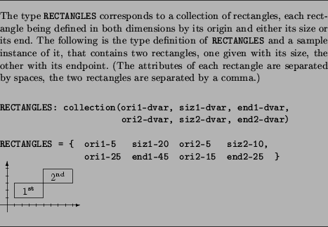
COLL: collection(c-collection(val-int))Such a data structure can be used to model different data in different constraints. Two of these are the following:
Keeping the notation of [8], which uses the name designator to refer to a sequence of names selected by slashes, let us introduce two new concepts, defined with BNF notation as follows:
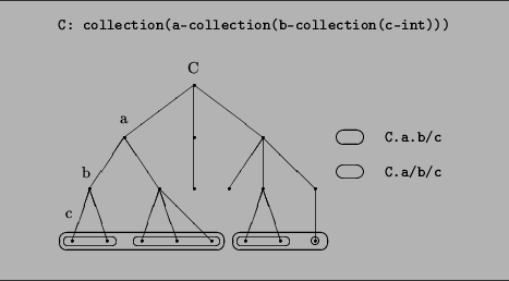
By starting a designator with a selector, we express that we want to divide the list of all the values into sublists and state something about these sublists separately. The division points are determined by the selector part of the designator. To clarify this, Fig. 5 shows a somewhat degenerated collection as a tree, along with two designators and the corresponding sublists marked with ovals.
In certain contexts only selectors are accepted. Among others, such places
are where the dot notation was already used, such as the argument of
required, or TABLE.index ![]() 1 in
Fig. 4. In the latter we want to express that all
values labeled as index must be greater than or equal to 1,
separately.
1 in
Fig. 4. In the latter we want to express that all
values labeled as index must be greater than or equal to 1,
separately.
Elsewhere designators are required. The argument of distinct is such a place. One would also use a designator to count those items of a collection which possess a certain attribute. Then one needs to write |COLL/attr|, because COLL/attr brings all the items with attr attribute together into a list, and | ...| returns the length of this.
Now let us return to the problem of distinct. In the example presented there, the statement distinct(COLL.c/val) means that for all c collections separately, the val values must be distinct, but the same value can appear in more than one collection (case 1). distinct(COLL/c/val), on the other hand, means that the list of all values in all collections must be distinct (case 2).
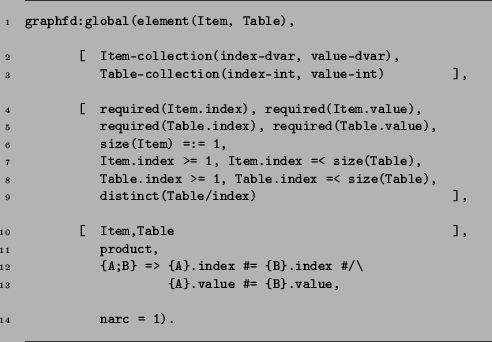
As stated in the introduction of Sect. 3, the chosen representation, while closely resembling the abstract syntax, follows the syntax of Prolog. Hence, each global constraint is described by a Prolog clause with seven arguments, as shown in Fig. 6 for the element constraint. These arguments are the following:
The lines of Fig. 6 correspond respectively to the lines of Fig. 4, and the definition as a whole should be self-explanatory. However, two things are worth mentioning.
One is that we have chosen to represent the arguments of the elementary constraint as items of a collection. In the body, we need to refer to these items and their attributes. However, there no syntax is defined to access the attribute of a single item of a collection, therefore we call for a trick. {A} means a collection with a single item (A), therefore {A}.index will expand to the index of this single element.
The other point to note that the relational operator #= comes from the SICStus CLP(FD) library, therefore, after expanding the selectors, the statement will become a valid CLP(FD) expression. The advantages of this will be discussed in Sect. 4.2.
The schema created by Beldiceanu allows us to test whether the relation expressed by a global constraint holds for a given set of concrete arguments. However, it does not deal with the more important case where only the domains of the arguments are specified, but their specific values are unknown. In such a case we need an algorithm to prune the domains of the arguments by deleting those values that would certainly result in a final graph not satisfying the properties. This question is fundamental in practical applications, therefore it is addressed by this section.
Development was launched with two goals in mind. The first task was to implement a relation checker, a realization of the testing feature offered by the schema, and a dumb propagator built on this checker. By and large, this task is finished, the results are presented by Sect. 4.1.
The second task was to implement an direct propagator capable of pruning variable domains based on an analysis of the current state of the graph, with the required properties in view. This task is much bigger, the development is still in an early stage. Its current state and features are introduced by Sect. 4.2.
Both tasks are implemented in SICStus Prolog [9], extending its CLP(FD) library by utilizing the interface for defining global constraints. This allows thorough testing of both the program and the theory itself in a trusted environment.
The first stage was to implement the complex relation checker, a program that checks whether the relation defined by the global constraint holds for a given set of values, but does no pruning at all. It includes the following features:
The checker was used to test the formal description of several constraints, whether they really conform to their expected meaning, and some errors in their specification have already been discovered (these will not be discussed here).
The second stage was to amend the relation checker with a generate-and-test
propagator. The idea is that whenever the domain of a variable changes,
all possible value combinations of the affected constraint's arguments are
tested with the relation checker, and only the values that passed the test
are preserved. This classical but extremely inefficient method for finding
solutions gives us full and exhaustive pruning.
The usage and output of the generate-and-test propagator is the same as that of the direct propagator, which is introduced in the next section (see Fig. 8).
Generate-and-test propagation is naturally out of the question in any practical applications. The direct propagator is the first step towards an efficient, applicable pruner. Here the line of thought is reversed: we assume that the constraint holds, and from the required graph properties we try to deduce conclusions regarding the domains of its variables.
To propagate the constraint, we have to look at this semi-determined graph and the required graph property together, and try to tell something about the still uncertain arcs. This process is called the tightening of the graph. In order to ensure that the graph properties hold, some of the uncertain arcs must be removed from the final graph, others must be made part of it. This causes the corresponding elementary constraints to be forced into success or failure, thus pruning the domains of the variables. The global constraint finally becomes entailed when there are no uncertain arcs left.
Because of the character of this propagation algorithm, elementary constraints are chosen to be reifiable CLP(FD) constraints, as already mentioned in the last paragraph of Sect. 3.2, an example of these is shown in Fig. 6. Reifiable constraints are connected with a Boole variable, and succeed if and only if the Boole variable has a value of 1. This use of reifiable constraints has several advantages. For one, a wide range of predefined constraints is available, already at this early stage of development. For another, the algorithm must be able to determine whether an elementary constraint holds or fails, or force it into success or failure, and the Boole variable linked to the reifiable constraints serves exactly that purpose.
To figure out how to tighten the graph at each step, that is, to find the rules of pruning, we need to study each graph property separately. There are simpler properties, such as prescribing the number of arcs, for which finding these rules is not very problematic (see below). A few of these are already handled by the propagator. The are more complex properties, like constraining the difference in the vertex number of the biggest and smallest strongly connected components, the pruning rules for these are a lot more complicated.
The current implementation can handle four graph properties, these are
narc, nvertex, nsource and nsink.
Fortunately, a large number of descriptions relies only on the first two,
thus many different constraints can already be propagated. Without going
into details, such constraints are among, disjoint,
common, sliding_sum, change, smooth,
inverse, and variants of these.
Current work is concentrated on the perfection of the propagation of these properties, and on the study of the nscc (number of strongly connected components) and related properties, which are also heavily used in the existing descriptions. The rest of the properties are only required by a minority of the constraints.
This propagator, although still not efficient enough to be useful in practical applications, may serve as a prototype for more effective implementations. A few thoughts on this issue are shared in the next section.
Pruning rules for more of the graph properties are to be worked out. The existing rules also need to be improved in certain cases. This will be the objective of an international project hopefully starting in Autumn 2003.
Using reifiable constraints as elementary constraints poses a problem: they do not necessarily provide a pruning as strong as expectable. Such a case can be seen on Fig. 9. What we see here, is that 1 is not excluded from the domain of A, although it could be. The problem is that forcing the and-ed elementary constraint of element (Fig. 6, lines 12-13) into failure is not enough to do that. We would get better pruning if we could write something like:
arc existsBut implication does not conform with the concept of elementary constraints. This problem requires further study.indices are equal
arc existsvalues are equal
Efficiency matters need to be considered more carefully when implementing further propagators. One way to increase efficiency, as suggested by Beldiceanu, could be to abandon the thought of a common propagator, that is able to parse such descriptions and prune in run time, and implement a pruner algorithm generator instead. This generator would take the description and convert it into a piece of code that does the pruning. This would shift the execution of complicated graph algorithms into compile time, where efficiency is a smaller issue. How this can be done must be worked out yet.
The paper began with the introduction of a theory first described in [8] that enables us to represent global constraints as regular graphs of the same elementary constraint. It was shown how the definition of a global constraint looks like, what restrictions and requirements may appear in it, and how the representative graph is built by it.
Then the concrete syntax of the language used by the implementation was presented. First, attention was drawn to two problems with the ADL specification, and solutions to them were suggested, too. Second, the concrete syntax itself was illustrated.
The last part of the paper introduced the actual results of my research through the programs developed as case studies. One of these was the complex relation checker capable of testing whether a constraint holds for a given set of values. The other, based on this, was the generate-and-test propagator, which implements exhaustive propagation for a large number of graph properties, but with very low efficiency. The result of the third, more interesting approach was the direct propagator, which was considered as a step towards efficient algorithms of constraint pruning. This deals with semi-determined constraint graphs and the enforcement of uncertain arcs in order to satisfy the required graph properties.
http://www.ilog.com. (2001)


![\begin{figure}\begin{Alltt}
Constraint: element(ITEM,TABLE)\par Arguments: ITEM:...
...M.value[1] = TABLE.value[2]\par Graph property: narc = 1\end{Alltt} \end{figure}](img15.png)
![\begin{figure}\begin{Alltt}[numbers=none]
Testing element(\{index-2,value-3\}, \...
...ld.
Graph properties failed.
Relation is not sustained.
\end{Alltt} \end{figure}](img19.png)
![\begin{figure}\begin{Alltt}[numbers=none]
\vert ?- graph_global(element(\{index-...
....
A = 1, B = 6 ? ;
A = 2, B = 2 ? ;
A = 3, B = 2 ? ;
no
\end{Alltt} \end{figure}](img27.png)
![\begin{figure}\begin{Alltt}[numbers=none]
\vert ?- graph_global(element(\{index-...
...ue-2 ; index-3,value-2\})),
B ...](img30.png)